

Machine learning offers a wide range of algorithms that differ in their principles and in their areas of use. For a beginner it can be hard to work out which algorithm to choose for a particular task. In this article I therefore introduce the common machine-learning algorithms in an accessible way, together with their practical use and a mutual comparison. We will go through classic methods such as logistic and linear Regression, decision tree, the k-nearest neighbours method (KNN), Support Vector Machines (SVM), naive Bayes classifier, artificial neural networks (ANN), but also unsupervised learning methods such as k-means clustering or principal component analysis (PCA). We will also add advanced ensemble methods including the random forest and boosting algorithms such as AdaBoost, Gradient Boosting (for example the implementations XGBoost or LightGBM).
Ensemble methods – the power of combination
Advanced approaches include ensemble methods, which combine several simple models (weak learners) into a stronger whole. The basic idea is that the errors of the individual models compensate for one another, which leads to better generalisation.
We distinguish three main approaches: bagging (Bootstrap Aggregating) trains several models independently on different subsets of the data and averages the results, thereby reducing the model’s variance. Boosting trains models sequentially, each new one concentrating on the errors of the previous ones, and reduces both bias and variance. Stacking uses a meta-model that learns to combine the predictions of different algorithms – the base models provide predictions that serve as inputs for the final meta-model. Stacking is particularly advantageous in competitions (Kaggle) and when combining heterogeneous base models (for example neural networks + XGBoost + SVM), where different algorithms capture different aspects of the data. In the following sections we will look both at the individual algorithms and at concrete implementations of these ensemble approaches.
The article explains what the individual algorithms are good for – for example which of them are used for classifying emails (a spam filter), predicting prices or recognising images. We will also compare the algorithms in terms of accuracy, computational demands (during training vs. during deployment), model interpretability and suitability for small vs. large datasets.
Why, in the context of AI, do we talk precisely about machine learning?
Artificial intelligence covers many approaches to solving complex problems. Traditional symbolic AI relied on expert systems with manually programmed rules, which worked for narrow domains but was brittle and did not scale. Automated planning and heuristic search (known for instance from chess programs) required detailed knowledge of the problem.
Machine learning brings a fundamental change – instead of programming rules by hand, the model learns from patterns in the data. This brings advantages such as scalability (more data usually means a better model), adaptivity (the model can be retrained on new data) and the ability to generalise to fuzzy or noisy cases. That is why ML dominates computer vision, natural language processing and recommender systems today.
Machine-learning algorithms and their practical use
Before we go into detail, it is worth realising that there are different types of machine-learning task. Classification and Regression are supervised learning tasks, in which the model predicts a known output (for example a category or a numerical value) on the basis of training data.
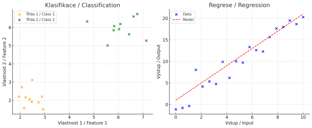
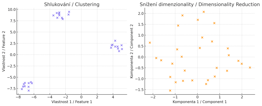
By contrast, clustering and dimensionality reduction are unsupervised learning tasks, in which the algorithm discovers structure in the data without predetermined correct answers.
When evaluating the performance of any algorithm it is essential to use cross-validation – a technique that divides the data into a training and a test part, in order to verify how well the model generalises to new, unseen data. This prevents overfitting and gives a realistic estimate of the model’s true accuracy.
Before training itself it is often necessary to pre-process the data. Standardisation or normalisation of input features is critical for algorithms sensitive to scale (KNN, SVM, neural networks, PCA), whereas tree-based algorithms cope with different scales without adjustment. Other common steps include dealing with missing values and transforming categorical variables.
When training models we encounter two basic problems: overfitting occurs when the model learns the training data in too much detail, including the noise, and cannot generalise well to new data. Conversely, underfitting means that the model is too simple and cannot capture even the basic patterns in the data.
These problems are related to the fundamental bias-variance trade-off . To mitigate overfitting, regularisation techniques that limit the complexity of the model are often used. Simple models usually have high bias but low variance – they are stable, but may be over-simplifying. Complex models have low bias but high variance – they can capture complicated patterns, but are sensitive to changes in the training data.
There are many metrics for evaluating models besides general “accuracy”. For Classification , precision, recall, the F1 score or ROC AUC are used, while for Regression it is MAE, MSE or R². The choice of metric depends on the nature of the problem – with imbalanced data, for example, accuracy can be misleading.
Below we list the most common algorithms with their description and examples of use.
Logistic regression (Logistic Regression)
Logistic Regression is a simple linear algorithm used mainly for binary classification (two-class problems). The model estimates the probability of belonging to a class using a logistic (sigmoid) function. In practice, logistic Regression is used, for example, for classifying emails as spam/ham, predicting customer churn (whether a customer will leave), or medical diagnostic tests (the probability of a disease on the basis of symptoms). Thanks to its linear character it is fast and scales well even to large datasets. The model is also easy to interpret – each input feature has a coefficient expressing its influence on the result, which makes it possible to understand how the model reached its decision.
| Advantages | Disadvantages |
| Logistic Regression is easy to implement and easy to understand. It provides a clear probabilistic output (for example “with a probability of 90 % this email is spam”). From a computational point of view it is a very efficient algorithm – training is fast and does not require large computing resources. It has a smaller capacity for overfitting than more complex models, but with a high number of features relative to samples, or with strongly correlated features, it can overfit. Regularisation (L1/L2) reduces this problem considerably. | The main limitation is the assumption of linearity - logistic Regression assumes a linear relationship between the input features and the log-odds (the logarithm of the odds ratio), which means the data should be linearly separable (separable by a hyperplane). In many real tasks this assumption does not hold.The model therefore cannot capture more complex non-linear relationships between inputs and output. A problem may also arise if the number of features is considerably greater than the number of training samples – in that case the model may overfit the training data. Logistic Regression also cannot directly handle multi-class tasks (either one-vs-rest schemes or softmax regression for several classes must be used). |
A typical use of logistic Regression
Classification binary events such as spam filters (spam vs. legitimate email – ham) or the detection of fraudulent transactions (fraud yes/no). It is also suitable for predicting probabilities, such as risk modelling in insurance or finance (the probability of loan default). It is also used in medicine for diagnostic tasks, for example the probability of a positive finding on the basis of tests.
Logistic Regression often serves as the default baseline model for comparison with more advanced algorithms, thanks to its simplicity and interpretability.)
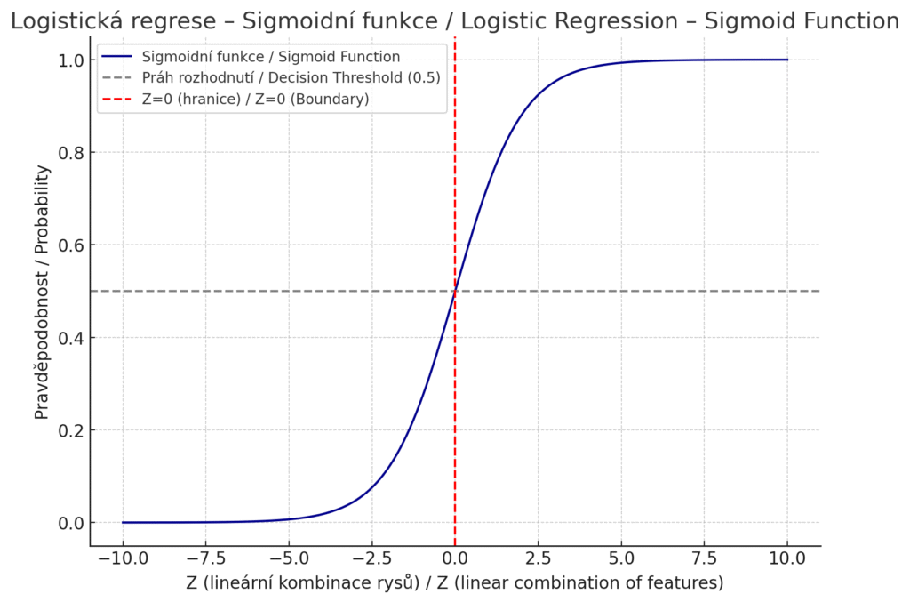
A graph of the sigmoid function, which forms the basis of decision-making in logistic Regression. It shows how the model’s linear output (the x-axis) is converted into a probability (the y-axis).
Linear Regression (Linear Regression)
Linear Regression is a basic algorithm for regression tasks, which models the relationship between the input features and a continuous target variable using a linear function. Unlike logistic Regression, which predicts the probabilities of categories, linear Regression directly estimates the numerical value of the output as a weighted sum of the input features plus a constant (the intercept). Mathematically it is written as y = β₀ + β₁x₁ + β₂x₂ + … + βₙxₙ, where the β coefficients are learned from the training data by the method of least squares. Linear Regression is widely used for predicting prices (property, shares), estimating sales, analysing the influence of marketing campaigns on revenue, or in economics for modelling relationships between macroeconomic indicators. Thanks to its simplicity it tends to be the first step in data analysis and serves as a baseline for comparison with more complex models, thanks to its simplicity and interpretability.
| Advantages | Disadvantages |
| Linear Regression is one of the fastest algorithms – both training and prediction are extremely fast thanks to the analytical solution (no iterative optimisation is needed). The β coefficients have a direct interpretive meaning – they show by how much the output changes when a given feature increases by one unit. The model is robust against overfitting, especially when regularisation is used (Ridge or Lasso Regression). It scales well to large data and does not require complicated hyperparameter tuning. It also provides statistical information about the reliability of the estimates (p-values, confidence intervals). | The main limitation is the assumption of linearity – the model can capture only linear relationships between inputs and output, which in many real situations does not hold. Linear Regression is sensitive to outliers, which can significantly distort the coefficients. It assumes homoscedasticity (constant variance of the errors) and normality of the residuals for correct statistical inference. With a high number of features relative to the number of samples, overfitting can occur. The model also suffers from multicollinearity – strongly correlated input features can cause unstable estimates of the coefficients. |
A typical use of linear Regression
Linear Regression is ideal for predicting continuous values where we assume approximately linear relationships. A common use is estimating property prices on the basis of floor area, location and the age of the building, predicting sales on the basis of marketing spend and seasonal factors, or analysing the influence of various factors on employees’ wages. In economics it is used for modelling relationships between GDP, inflation and unemployment. In scientific research it helps to quantify relationships between variables – for example the influence of temperature on plant growth. If a linear model achieves good results, it may be a better choice than more complex algorithms because it is easy to explain and deploy. If linearity is not enough, the model can be extended with polynomial features or interactions between variables, or one can move on to more complex algorithms.
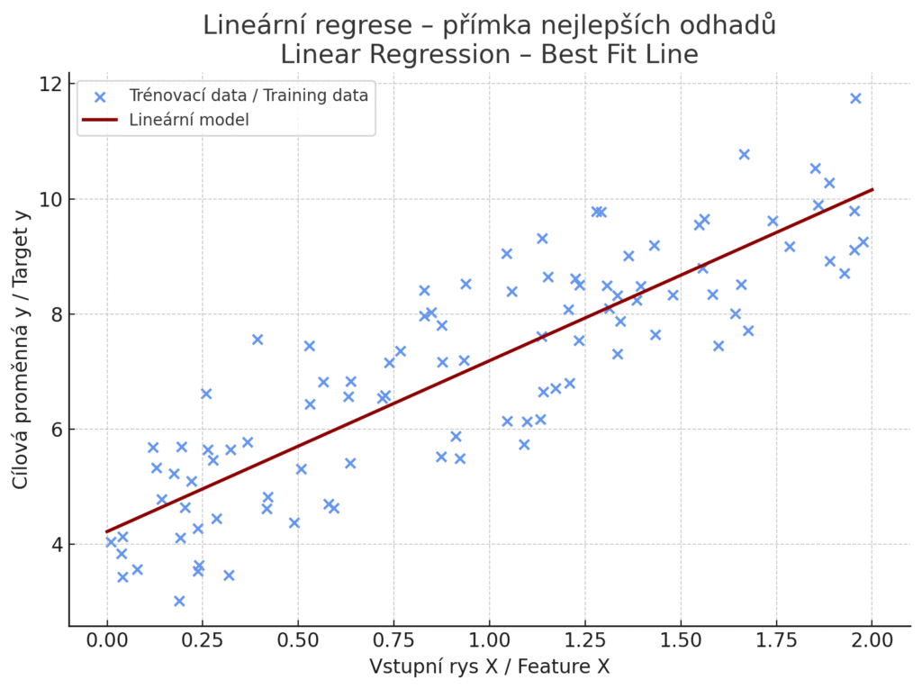
The blue points represent the training data – inputs and the corresponding outputs. The red line is a linear model of the form y=β0+β1x, trained by the method of least squares. The model tries to minimise the total squared difference between the predictions and the actual values.
Decision tree (Decision Tree)
Decision trees are popular interpretable models for both classification and regression. The tree gradually divides the data according to the values of the input features – at its nodes it asks “decision questions” of the type “Is the value of feature X > 5?” and branches further according to the answer. The result is a tree structure in which the leaves represent final decisions or predictions. A decision tree can capture non-linear relationships between the input variables and the target. Thanks to the tree structure its decision-making is easy to explain: it can be visualised and one can follow the path from the root to a leaf, which represents the decision rules leading to the conclusion. This is useful when decisions have to be defended – the result can easily be interpreted and justified.
| Advantages | Disadvantages |
| The main advantage is the simple interpretation of the resulting model – even a non-technical user can follow the rules in the tree and understand why the model arrived at a given prediction. Decision trees can work with various types of input (both numbers and categories) and do not require feature scaling. They can also handle non-linear relationships and interactions between variables (unlike purely linear models). Training a tree is relatively fast even on larger data, because the algorithm searches through splits of the data according to individual features and selects the most informative splitters. | A simple tree has a tendency to overfit the data if it is allowed to grow freely to a great depth. Deep trees may create very specific rules that hold only for the training data, and thereby lose the ability to generalise to new data. That is why the depth of the tree or the number of samples in the leaves is often limited in order to improve generalisation. Decision trees also suffer from high variability – small changes in the data can lead to a completely different tree structure. A single tree tends to have lower predictive accuracy than more sophisticated methods (for example ensemble methods such as random forest or boosting, which use many trees). With imbalanced data (class imbalance) trees may favour the majority class and neglect minority classes. |
Typical uses of decision trees
They are used for decision processes, where the tree can represent a procedure for deciding on the basis of input parameters (for example approving a loan according to the client’s income and history). They are also used in medicine, as diagnostic trees for recommending treatment on the basis of a patient’s symptoms (easily interpretable for a doctor). They are also suitable for rapid prototyping: trees can be used for quick exploratory data analysis – they reveal which variables have an influence and which threshold values are critical (they also help with feature selection).
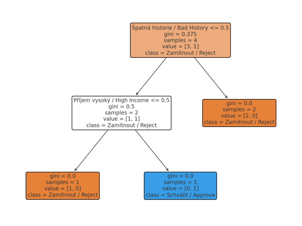
A decision tree showing the loan approval process on the basis of two input parameters – income: high vs. low / credit history: good vs. bad. The visualisation shows how the tree asks decision questions and arrives at a final decision: approve or reject.
Random forest
Random forest is an ensemble method built on decision trees. Instead of a single tree, the algorithm trains a large number of trees (a forest) on different subsets of the data and different selections of features. Each tree in the forest votes for its result and the random forest decides by majority vote (Classification) or by averaging the predictions (Regression). This principle of bagging (bootstrap aggregating) with a random selection of features ensures that the trees are mutually diverse and that the model does not overfit as easily as a single deep tree. Thanks to the combination of many trees, a random forest usually achieves high accuracy and is robust against noise in the data.
| Advantages | Disadvantages |
| A random forest typically provides very accurate predictions thanks to averaging many models, which reduces their variance and improves generalisation. It is resistant to noise and outliers in the data; individual trees may pick up part of the noise, but the majority of the trees outvote any erroneous learned patterns. The model can estimate the importance of features – from the frequency of use or the deterioration of the error after permuting a feature one can infer which inputs are most significant for the prediction. This is valuable for interpretation at the level of the whole dataset (even though the decision process for individual predictions is not as transparent as with a single tree). | The interpretability of a random forest is limited – it contains hundreds or thousands of trees, which a human can no longer examine in full (though feature importance can be used, or individual trees can be inspected). The computational demand is higher than for a single tree, especially during training – the model trains many trees (100 or 1000, for example) and that requires more time and memory. At deployment (inference) the model has to evaluate every new example in all the trees, which can be slower (but can still be parallelised, because the computation in the different trees is independent). With very large datasets (millions of samples) training a random forest can become lengthy and memory-intensive – in such cases more efficient boosting algorithms are often chosen. The key hyperparameters include the number of trees (n_estimators), the maximum depth of the trees (max_depth) and the number of features for each split (max_features). |
Typical uses of random forests
These are above all predictions on structured data. The random forest is a popular default algorithm for tabular data in areas such as financial models, industrial prediction, bioinformatics (for example predicting diseases from genomic data) and so on. If you are solving tasks with a large number of features, then thanks to the built-in estimate of feature importance it is used for selecting the most influential inputs. In medicine, for example, it helps to determine which factors (symptoms, laboratory values) most influence a diagnosis. Another field of use is applications requiring robustness– in an environment with noise or missing data (for example IoT sensors with dropouts) the random forest, thanks to averaging, copes better with poor-quality data.
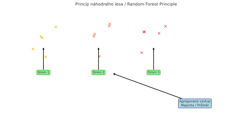
How a random forest works – three random bootstrap samples of the data (top), three trained trees, each with a different view of the data, aggregation of the output by voting or averaging.
The nearest neighbours algorithm (K-Nearest Neighbors, KNN)
K-Nearest Neighbors is a simple memory-based algorithm which, for a new input, looks for the closest training examples in feature space and derives a prediction from their values. For Classification it lets the new point “vote” among its k nearest neighbours: it assigns it the class that is most frequent among the neighbours. For Regression the average of the neighbours’ values is often taken. KNN is a so-called lazy learning algorithm – there is no explicit training phase, the model merely remembers the training data. This means that new samples can be added easily without having to retrain the whole model.
| Advantages | Disadvantages |
| The method k of nearest neighbours is conceptually simple and easy to understand. It does not require complicated optimisation processes – for a new point it is enough to compute the distances to the training points. Because there is no explicit training, it does not learn parameters; the choice of k works as a regularisation mechanism – a small k (especially k=1) leads to high variance and overfitting to local noise, while a large k reduces variability but may cause boundaries that are too smooth. KNN is flexible – it can handle multi-class Classification and with different distance metrics (Euclidean, Manhattan, Minkowski) its behaviour can be adapted to a particular problem. It can also be used for recommender systems (for example recommending a product to a user on the basis of similarity with other users). | The computational demand at deployment grows dramatically with the size of the training set. If we have thousands or millions of training points, finding the nearest neighbours for each query can be slow (the distance to all points has to be computed). There are structures that speed this up (a k-d tree, for example), but in high dimensions their benefit disappears. The model also requires storing the whole training dataset in memory, which can be demanding. KNN is also sensitive to scaling and noise – different ranges of features affect the distance metrics (inputs have to be normalised) and outlying or noisy points can have a disproportionate influence on the prediction. KNN decides by majority vote among the neighbours, and k=1 means zero training error (the model “remembers” every training point), which leads to overfitting to local noise. Conversely, a large k can blur the boundaries between classes. |
Typical uses of K-Nearest Neighbors
For example the classification of Classification images or patterns with small datasets – a new image can be classified according to which known images it is closest to in its properties (colours, textures and so on). It is used in recommender systems (Spotify, Netflix, product recommendations in an e-shop), because KNN can be applied to a matrix of users and items – finding the “closest” users with a similar taste and recommending items that a neighbour liked, or analogously with items (so-called user-based or item-based collaborative filtering). It is also used for various anomalies and outlier detection – points that have no close neighbours (the distances to the nearest ones are high) can be regarded as outlying or suspicious (fraud detection, for example).
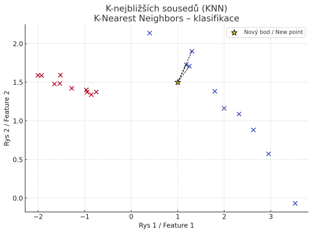
A simple visualisation of the principle of K-nearest neighbours (K-Nearest Neighbors) in a graph – the coloured points are training samples, the gold star is the new point we want to classify, and the dashed lines connect the new point with its three nearest neighbours.
Support Vector Machine (SVM)
Support Vector Machine (SVM) is a powerful algorithm for classification (and also regression), known for looking for the so-called optimal hyperplane separating the classes. The goal of an SVM is to maximise the margin – that is, the distance of the nearest training points from the separating plane. Intuitively it tries to find a boundary that best separates the classes and at the same time has the greatest possible distance from both classes, which improves generalisation. A key property of SVMs is support for kernel functions (the kernel trick), which make it possible to transform the input data into higher dimensions, where they are more easily linearly separable. In this way an SVM also copes with non-linear classificationif we choose a suitable kernel (RBF, polynomial and others). SVMs were popular above all in the era before the arrival of deep learning – they achieved top results in image recognition (a well-known application is the recognition of Classification handwritten digits) and in text classification.
| Advantages | Disadvantages |
An SVM is efficient in high-dimensional spaces with a small number of samples - training scales from O(n²) to O(n³), so it works well when the number of features is high relative to the number of samples. For millions of samples, however, it is unusable. It also has a good ability to generalise; thanks to maximising the margin it is not as prone to overfitting as, for example, a decision tree. An SVM with a suitable kernel can achieve good results high accuracy even on complex tasks, especially if a medium-sized dataset is available. It is versatile – it allows various kernels and thus the solving of diverse problems (linear separation, non-linear boundaries, and with a suitable kernel even problems such as sequential data). | Training an SVM is computationally demanding, especially for large datasets. The classic SVM solves a quadratic optimisation problem that scales from O(n²) to O(n³) with the number of samples – for tens of thousands of samples or more, training can be very slow. There are linear variants of SVM and stochastic methods that scale better, but for non-linear kernels this is a limitation. An SVM also requires hyperparameter tuning – choosing a suitable kernel and parameters (the regularisation parameter C, the gamma parameter of the RBF kernel) is not trivial, and a poor choice can significantly worsen performance. The interpretability of an SVM is limited – with a linear SVM the weights can be interpreted similarly to logistic Regression, but with non-linear SVMs in kernel space the model is perceived as a black box. Moreover, the resulting decision functions of an SVM are determined by so-called support vectors (a subset of the training points), whose combination defines the boundary, which again makes it harder to explain a prediction. |
Typical uses of the Support Vector Machine
SVMs (often linear SVMs) are successfully used for categorising text documents (spam detection, sorting articles by topic) thanks to their ability to work with many attributes (words). Before the arrival of deep neural networks, SVMs with a non-linear kernel were state of the art in, for example, handwriting recognition (the well-known MNIST data) or object detection in images. They are also used in the analysis of genetic data or the classification of proteins, where the data points are in a very high dimension and a robust classifier is needed for a small number of training samples.
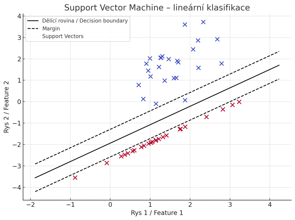
A visualisation of the principle of the Support Vector Machine (SVM) with a linear kernel – the black line is the optimal separating plane, the dashed lines show the edges of the margin, and the empty points with a black outline are the support vectors, the samples that determine the position of the decision boundary.
Naive Bayes classifier (Naive Bayes)
Naive Bayes is a simple probabilistic classifier based on Bayes’ theorem. It is called “naive” because it makes the strong (and often unrealistic) assumption that the input features are conditionally independent within each class. In practice there are several variants (multinomial, Bernoulli, Gaussian naive Bayes) according to the type of data they process. Despite its simplifying assumptions, naive Bayes tends to be surprisingly effective, above all with text data. In document classification (spam filters, sentiment analysis) it works decently, because the words in a document can be regarded as more or less independent with respect to the class (spam emails, for instance, often contain certain words independently of one another). From the training data the model computes the probabilities of the occurrence of features (words) in the individual classes, and when predicting it selects the class for which the combination of features is most probable.
| Advantages | Disadvantages |
| Naive Bayes is very fast both in training and in prediction – essentially it is enough to go through the training data and count the frequencies of occurrences of combinations of features and classes. Thanks to this it makes few demands on computing power and can easily scale to large volumes of data. Surprisingly, it also works well with little training dataif the independence assumption happens to be roughly satisfied – it can generalise even from a few examples thanks to incorporating prior probabilities. A large number of input features (thousands of words in a text, for example) does not bother it; on the contrary, it is one of the algorithms that cope with high dimensionality (often better than more complex models). | The main disadvantage is the already mentioned assumption of feature independence – in real data, features are typically not entirely independent, and naive Bayes does not know how to take their dependencies into account. This can lead to less accurate predictions if the correlations between the inputs are important. Another practical problem is the so-called zero-frequency phenomenon: if a particular combination of feature and class does not occur in the training data at all, the model assigns it zero probability, which then nullifies the probability of the whole prediction. The solution is to use so-called smoothing, which adds a small constant to the counts and prevents zero probabilities. Naive Bayes is also not a good estimator of the probabilities themselves – its output probabilities tend not to be calibrated (it is often too confident), so it is more suitable simply for determining the most probable class. Interpretation of the model is possible from the point of view of probabilities (we can see which features are most significant for a given class – which word most “signals” spam, for example), but because of the independence assumption it may be misleading and is not as straightforward as with a decision tree, for instance. |
Typical uses of Naive Bayes
Naive Bayes was historically the core of many spam filters, and it is also used for sorting articles, emails or news by topic or sentiment. Thanks to its speed it is suitable where decisions have to be made immediately – filtering harmful web pages in a browser, detecting inappropriate comments and so on, especially if the inputs are represented simply (as word vectors, for example). Because it naturally supports multiple classes, it can also be used where we have dozens of categories (sorting newspaper articles into sections, for example).
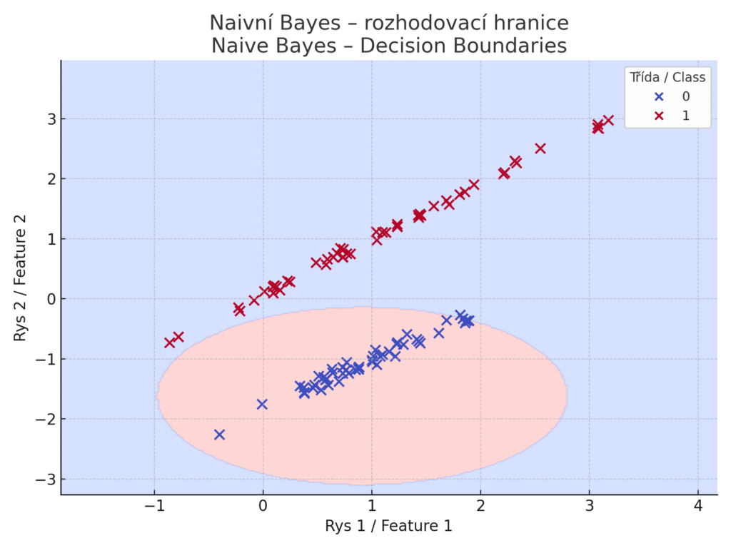
The model expects every feature to have a normal distribution within each class and the features to be independent of one another. The blue area – for any point in this area the model would predict Class 1 (“positive”, “spam”, “yes”…). The coloured areas show the decision boundaries, which follow from the computation of probabilities. The points represent training samples of two classes. The red area – for a point in this area the model would predict Class 0 (“negative”, “ham”, “no”…). Unlike decision trees or linear Regression , naive Bayes does not have sharp straight boundaries, because it decides on the basis of a continuous probability – and the Gaussian distribution is bell-shaped.
Artificial neural networks (ANN)
Artificial neural networks (ANN) represent a whole family of models inspired by the working of the brain. They consist of interconnected neurons (nodes) arranged in layers. Deep neural networks (deep learning) have several hidden layers, which allows them to learn very complex functions.
Popular architectures include feed-forward networks (used for tabular data), convolutional neural networks (CNN) for image processing, and recurrent networks (RNN) and transformers for sequential data (text, time series). Neural networks excel at representation learning – they can automatically extract and combine suitable features from the data in their hidden layers. Thanks to this they achieve top accuracy in many tasks, provided enough data is available. In image and sound recognition , for example, deep networks today significantly outperform classic algorithms; they are the basis for technologies such as self-driving cars (recognising the surroundings with cameras and LIDAR), voice assistants (speech recognition, machine translation) and object detection in video.
| Advantages | Disadvantages |
| Artificial networks are among the most powerful models in terms of predictive accuracy. They can learn very complex non-linear relationships in data that other algorithms would not capture. They are versatile – with a sufficiently large network any function can theoretically be approximated (the universal approximation theorem). In many domains neural networks hold the current records; for example CNNs in computer vision for image classification (ImageNet) or transformer models in NLP (translation, language models). Another advantage is that the network learns directly from the raw representation of the data – in image recognition, for instance, there is no need to design features by hand, since the network itself learns to detect edges, shapes and objects in its various layers. Scalability is another plus: with enough computing power one can train on enormous datasets and keep improving the model (powerful hardware such as GPUs/TPUs is, however, a necessity). | The biggest pitfall of neural networks is the need for a large amount of training data. Networks have a huge number of parameters that have to be learned – modern deep models have millions to billions of weights. If we trained them on a small dataset they would almost certainly overfit. That is why they are used mainly where extensive datasets are available or where pre-trained models can be used. The computational demand is also very high: training a deep network can take hours or weeks on powerful graphics cards. Deployment (inference) can also be slow, especially with large models, though this can be improved by optimisations and specialised hardware (accelerators). The interpretability of neural networks is low – this is the typical “black box”, in which millions of parameters have no meaning comprehensible to a human being. There are explanation methods (visualising activations, LIME, SHAP), which can provide a certain insight, but in general it is very difficult to explain why a network made a particular decision. In some areas networks also run into a stability problem – tiny changes in the input can cause a completely different prediction (a well-known example is adversarial examples in images, which fool even otherwise accurate CNNs). |
Typical uses of neural networks
Neural networks are currently known above all for natural language processing (NLP). Language models such as GPT for text prediction, machine translation and speech recognition (converting spoken speech into text) – all of this is now handled by deep neural networks (RNNs, transformers). Another use is in the field of computer vision, such as the classification of Classification objects in images (recognising animals in photographs, for example) or the detection and segmentation of objects in video (recognising pedestrians and cars for autonomous driving, for example).
They are also suitable for predictions on tabular data. Neural networks can be deployed even in ordinary tasks such as price prediction or fraud detection, especially where there is a lot of data – and yet simpler models or ensembles such as boosting, which can be more efficient, are often used here too.
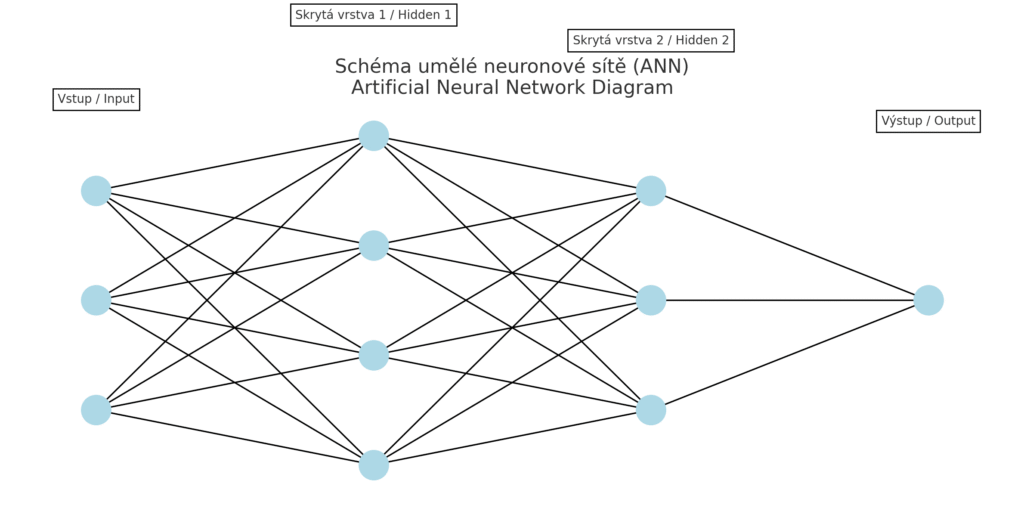
The diagram of a neural network shows three inputs, two hidden layers and one output. All the layers are fully connected – every neuron is joined to all the neurons in the next layer. It illustrates the principle of a feed-forward neural network, often used for tabular or structured data.
K-means clustering
K-means is the best-known algorithm for cluster analysis (clustering), that is, for finding natural groups in data without predetermined categories. The aim of k-means is to divide the data into k clusters in such a way that the points in one cluster are as similar to one another as possible (as close as possible in space) and at the same time far from the points in other clusters. The algorithm works iteratively: it randomly chooses k initial cluster centres, assigns each point to the nearest centre and then recalculates the centres as the average of the points in the cluster. It repeats this process until the centres settle. The result is the coordinates of the centres (so-called centroids) and the assignment of each point to one of them. The uses of k-means are in tasks where we want to discover latent groups – segmenting customers according to purchasing behaviour, clustering images according to visual similarity, grouping documents with similar topics and so on.
| Advantages | Disadvantages |
| K-means is a relatively simple algorithm with a time complexity of O(n·k·d·i), where n is the number of points, k the number of clusters, d the dimension and i the iterations. For small and medium data it is fast, but as any of the parameters grows (especially n or k) it can become slower. For very large datasets optimisations such as MiniBatch K-means are used. With a sensibly chosen k and initialisation it converges within a few iterations (although there is a risk of converging to a local minimum). The algorithm is easy to implement and to understand, which makes it a frequent choice for an initial exploration of data. For new (unseen) points the assignment to a cluster is very easy and fast – it is enough to compute the distance to the k centroids and choose the nearest one. | With k-means it is necessary to choose the number of clusters kin advance, which need not be obvious, so several values are often tried. The algorithm is sensitive to the initial choice of centroids – a poor initialisation can lead to worse results (this is partly prevented by clever initialisation such as k-means++). K-means also works best if the clusters have an approximately spherical (convex) shape and a similar size; with data containing irregularly shaped clusters it can fail, because it always optimises only intra-cluster distances. The algorithm is also sensitive to outliers – even a single outlier can shift a centroid considerably. In high-dimensional spaces k-means often suffers from the so-called curse of dimensionality – the distance metric loses its explanatory power and all the points may be roughly equally distant. This reduces the quality of the clustering. Interpreting the clusters can be demanding: k-means itself does not say what characterises the clusters, it merely divides the data. The analyst has to interpret the meaning of the groups found afterwards (“cluster 1 consists of customers who frequently buy small items”, for example). |
Typical uses of k-means
- Customer segmentation: On the basis of data about customer behaviour (purchases, frequency, demographics), k-means can divide customers into groups for targeted marketing.
- Image processing: K-means is used for colour quantisation – one chooses k colours that best represent the image, and the other colours are replaced by the nearest centres. In this way an image can be compressed (fewer colours) or segmented into areas according to colour.
- Initialisation for other algorithms: Centroids from k-means can serve as an initial representation of the data (in feature learning, for example), or as initial states for more complex models (initialising the centres in a GMM, for instance).
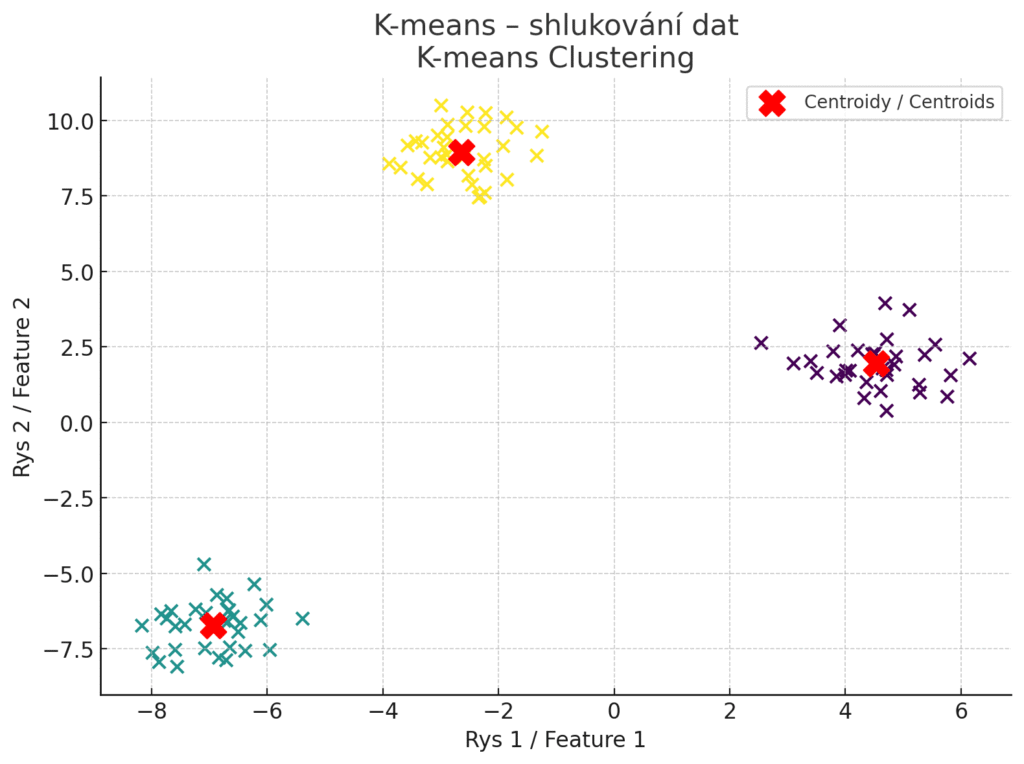
A visualisation of how the K-means algorithm works. The coloured points show the individual data points divided into three clusters. The red “X” marks represent the centroids – the average positions of the points in each cluster. Every point is assigned to its nearest centroid, so that compact and well-separated groups are formed.
Have you noticed that at first sight the algorithms K-means and K-nearest neighbors (KNN) may seem similar? Both are often visualised as points spread out in space, divided according to a certain proximity or membership of a group. In both cases, moreover, people talk about “nearest points”, “clusters” and measuring distances. But beneath the surface these two approaches are fundamentally different – in purpose, in the way they work and in their use. K-means is an algorithm of unsupervised learning. There are no previously known classes or categories. The aim is to find natural groups (clusters) in the data. The algorithm itself works out which points are similar and groups them into clusters so that the points in one cluster are as close to one another as possible and as far as possible from the points in other clusters. KNN , by contrast, belongs to supervised learning. It works with training data in which the class of every point is known. When classifying a new point the algorithm looks at which known samples it is closest to and determines its class by majority vote.
In visualisations both models may look similar: the data are divided in space and colour-coded. But:
- K-means divides the space on the basis of proximity to the centre of a cluster – the areas tend to be even and symmetrical, because the centroids are geometric averages.
- KNN divides the space unevenly, according to where the known points actually lie – the boundaries are often jagged and complicated, because they respond to specific local patterns
Principal Component Analysis (PCA)
Principal component analysis (PCA) is a basic method for reducing the dimensionality of data. Its aim is to find a new set of orthogonal variables (principal components) that capture as much of the variability of the original data as possible. In practice this means finding the direction in the data space in which the data are most spread out – that will be the first principal component. The second principal component is the direction with the second largest variance, which is at the same time perpendicular to the first, and so on. By projecting the data into the first few components we thus obtain a smaller number of new features which nevertheless still capture most of the information from the original data. PCA is widely used as data pre-processing – reducing the dimension can remove noise and redundant information, speed up the subsequent training of models and sometimes even improve accuracy (if the filtered-out noise had previously confused the model). It is also used for data visualisation – by projecting high-dimensional data into 2D or 3D (the first two or three components) the data can be displayed and structures observed (clusters, outliers).
| Advantages | Disadvantages |
| PCA removes correlated features – the new components are linear combinations of the original features, and it can thus merge information from strongly correlated variables into one. This both reduces redundant data and can improve the performance of some models (linear models or k-means, for example, can suffer from multicollinearity, which PCA eliminates). Reducing the dimension also limits overfitting – in a smaller parameter space a model cannot overfit the noise so easily. PCA is computationally feasible even on relatively large data thanks to efficient implementations (SVD, for example). Deployment of PCA (projecting new data) has a time complexity of O(d × k), where d is the original dimension and k the number of components – projecting from 1000 features into 10 components significantly speeds up the subsequent computations. | Interpreting the principal components is not always easy – each component is a combination of the original features and need not have a direct semantic meaning. It is, however, possible to analyse which original features contribute most to the individual components (loading vectors), which helps to understand what a component represents. The first component, for example, may represent a combined “general factor” covering several original quantities, which is hard to put into words. When PCA is used there is also a loss of information – if we select only the first few components, we neglect the rest of the variance (however small). This can be a problem if information important for certain rare cases happens to lie in the neglected part of the space. PCA also assumes linearity – it looks for linear combinations of features. If non-linear relationships are the important ones, there are better methods ( t-SNE, UMAP for visualisation, or autoencoders in deep learning for non-linear dimensionality reduction). From a practical point of view it is necessary to standardise the input data before PCA – the variance metric is affected by scale, and features with larger numerical values would dominate the selection of components. |
Typical uses of PCA
Before training more complex models (SVM, neural networks) on data with many features, PCA is used to reduce the dimension and filter out noise, which speeds up training and potentially improves performance. In genetics PCA helps to visualise high-dimensional data such as the relatedness of populations (projecting genomic variation into 2D), in economics to display markets, and so on. PCA can be used for data compression – for an image, for instance, the principal components (eigenimages) can be found and only the coordinates of the point in component space stored instead of the original pixels.
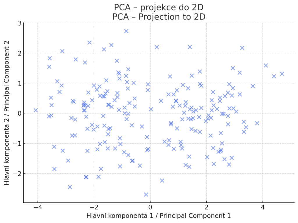
A visualisation of the result of principal component analysis (PCA). The data were originally in a 5-dimensional space. Using PCA they were projected down to 2D, with the retained axes (PC1 and PC2) representing the two directions of greatest variance in the data. This visualisation reveals any clusters, outliers or geometric structure of the data in the main directions of variability.
Self-Organizing Maps (SOM, Kohonen networks)
Self-Organizing Map (SOM) is a specific type of neural network designed for unsupervised learning, which makes it possible to transform high-dimensional data into a two-dimensional representation. Its strength lies not only in its ability to classify or cluster, but above all in the fact that it preserves the topological arrangement: similar samples remain close to one another even after the projection. In this the SOM differs fundamentally from K-means, for example, which does group similar data but does not preserve their mutual relationships in space.
The input can be any number of features – a vector of size 50, for example, may represent a customer, a gene expression or a network flow. Behind it there is a grid of neurons (often 2D, for instance 10×10), where each neuron has a weight vector of the same length as the input data. Training proceeds by repeatedly going through the inputs, during which we first find the nearest neuron (the so-called Best Matching Unit – BMU) for a given input vector, then update the weights of this neuron and its neighbourhood so that they move closer to the input sample, and reduce the influence of the neighbourhood and the learning rate over time.
The result is a map in which similar inputs end up close to one another, which gives rise to a natural segmentation and a spatial structure.
| Advantages | Disadvantages |
| Excellent for visualising complex data, preserves topology, relatively fast training O(n × epochs), makes it easy to identify clusters and anomalies through heat maps. | Sensitivity to the choice of grid size and initial weights, difficult interpretation of what the individual areas of the map represent, less accurate than specialised clustering algorithms. It cannot easily be used for prediction; it is exclusively a tool for exploration, not for supervised learning. |
Typical uses of the Self-Organizing Map
Customer segmentation with a visualisation of their characteristics, analysis of genomic data, detection of anomalies in network traffic through heat maps of deviations, exploratory analysis of high-dimensional data before applying other algorithms.
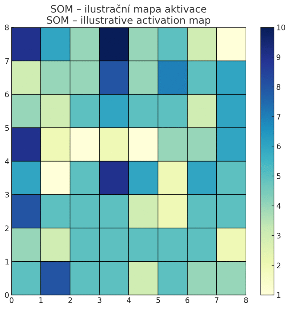
An illustrative visualisation of a Self-Organizing Map (SOM), in which every field of the 2D grid (8×8) represents one neuron. The intensity of the colour shows how many input samples “fell” into a given neuron – the darker it is, the more data points were assigned to it. This map helps one to sense intuitively where the clusters, the dense areas and the outlying areas (with low activity) are.
AdaBoost (Adaptive Boosting)
AdaBoost is the first popular algorithm from the family of boosting methods. Boosting in general works by sequentially adding several simple models to the combination (weak learners), with each new model concentrating on the errors of the previous ones. AdaBoost in particular often uses as weak learners simple decision trees (so-called stumps – trees of depth 1 or 2). It gradually trains a small tree, evaluates the errors, increases the weight of the incorrectly classified samples, and in the next tree these harder cases have greater influence. In this way the ensemble “adaptively” improves on the more difficult examples. The final prediction is then a weighted combination of all the weak models (for Classification usually voting with the weights α, for Regression a sum). AdaBoost became famous in the task of detecting faces in images (the Viola-Jones algorithm), where a combination of many simple rules was able to detect faces effectively in real time.
| Advantages | Disadvantages |
| AdaBoost typically increases accuracy compared with a single tree – by combining many weak rules a strong model can be obtained. It is less prone to overfitting than a large deep tree, because it regularises the weak learners – each small tree is very simple and on its own would have a large error, but in combination the errors compensate for one another. At the time it appeared, AdaBoost was popular for its easy implementation and interpretation – the weak trees (stumps) could be visualised and the weights α showed the importance of the individual trees, which gave a certain insight into the model. | AdaBoost is sensitive to outliers – if the training data contain incorrectly labelled examples or outliers, boosting will try at all costs to learn them (giving them growing weight), which can worsen the overall performance. The algorithm is also not trivially parallelisable, because new weak models build on the results of the previous ones – this can be a disadvantage with really large datasets. In such cases training can take a long time (thecomputational demand grows with the number of iterations/weak models). AdaBoost itself does not have many free parameters, but setting the number of iterations, for example, is important – too many weak models can lead to overfitting, too few to underfitting. Today the original AdaBoost has been surpassed by more advanced boosting algorithms (see below), which scale better and are more robust. |
Typical uses of AdaBoost
As already mentioned, AdaBoost became famous in face detection (it combined simple Haar features). In general, boosting can be used for any object detection in which many simple rules are combined. AdaBoost can be applied to a wide range of classification tasks instead of logistic Regression or SVM, if the aim is higher accuracy and longer training is not a problem. In practice, however, it is today often replaced by its more advanced version, gradient boosting. In earlier machine-learning competitions (Kaggle around 2010) AdaBoost was one of the ensembles that could be tried in order to improve a model’s accuracy. Today it has been eclipsed by algorithms such as XGBoost.
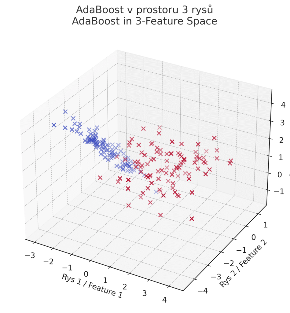
A 3D visualisation Classification using AdaBoost on data with three input features. This is a 3D arrangement of the predicted classes, not a decision boundary (that can no longer be displayed directly in 3D without complicated grid slices). Each point is shown in the space according to the values of the three features. The colour shows the output of the prediction (two classes).
Gradient boosting (XGBoost, LightGBM and others)
Gradient boosting is an improvement on the idea of AdaBoost – instead of penalising errors with data weights, boosting is treated as a sequential optimisation by gradient descent in function space. Without going into detail, this means that the new weak models are trained so as to approximate the gradients of the errors of the previous ensemble (that is, they learn directly from the residual errors). Decision trees are typically used as the weak models here too, but they can be deeper than stumps.
The result is a very powerful ensemble model known as Gradient Boosted Trees (GBDT). Specialised libraries have established themselves that implement gradient boosting extremely efficiently – above all XGBoost and LightGBM (another is CatBoost). These algorithms dominate many competitions and applications, especially on structured tabular data, where they often outperform even neural networks in the performance/computation ratio.
XGBoost (Extreme Gradient Boosting)
This is a popular open-source library that brought a whole range of optimisations to boosting. XGBoost implements L1/L2 regularisation to limit overfitting, uses parallel computation (it trains several branches of a tree simultaneously) and an efficient way of pruning trees. It can also handle missing values elegantly (it decides itself which branch to send them to).
XGBoost became famous in the data-competition community – it became the go-to algorithm on Kaggle, where it won many competitions. But it can also be found in industry, for example in financial models (risk prediction, fraud detection) or in healthcare, where high prediction accuracy is needed. Thanks to its robustness it is also used for anomaly detection.
LightGBM
A library from Microsoft that speeded up boosting by means of the so-called histogram method of learning. Instead of going through all the possible thresholds of continuous variables (which is demanding with trees), LightGBM converts the values of features into adaptive histograms and works with these bins. This significantly speeds up training and reduces memory requirements, especially on large data.
LightGBM also uses an innovative way of growing a tree, so-called leaf-wise (it first expands the leaf with the greatest improvement), which can lead to deeper specialised trees, but with a parameter for limiting overgrowth. Another advantage of LightGBM is native support for categorical variables (they do not have to be one-hot encoded). It is used in applications where there are large volumes of data and a requirement for speed – for example real-time predictions in online systems (advertising auctions, recommendations). LightGBM can quickly process even huge datasets, where other algorithms would be slow or would not fit into memory.
| Advantages | Disadvantages |
| Modern boosting algorithms achieve top accuracy on many tasks. They combine the strengths of trees (non-linear modelling, working with different types of data) with the power of an ensemble. Compared with a random forest they often optimise the error better – each new tree purposefully reduces the residual error, which leads to higher accuracy with fewer trees. XGBoost and LightGBM are, moreover, very efficient implementations – they use parallelism, optimised data structures and tricks for speed. They also support a great many settings for regularisation (the maximum depth of the trees, learning with subsampling of the data or features, penalising the complexity of the trees) in order to control overfitting. Another advantage is robustness – they can cope with missing values and often do not require extensive prior adjustment of the data (normalisation, for example). | The price for the performance is a higher computational demand during training – boosting is sequential, each new tree waits for the results of the previous ones, which limits parallelisation compared with a random forest. Training can be slower, especially if many iterations are required (hundreds to thousands of trees). Memory requirements can grow with large data (XGBoost is known for potentially consuming a lot of memory with the default settings; LightGBM is more economical in this respect). The interpretability is again low – although we can examine feature importance and the individual trees, overall the model is composed of many components and its decision-making is not transparent. For deployment, prediction is slightly slower than with a single tree, but if the number of trees is reasonable (hundreds), it is still manageable even in real time. In general, gradient boosting can overfitif, for example, too many trees or too great a depth are used without sufficient regularisation. That is why it is important to tune the hyperparameters carefully. |
Typical uses of gradient boosting
Gradient boosting (mainly XGBoost, LightGBM, CatBoost) is often a key part of winning solutions in machine-learning competitions for tabular data – predicting property prices, Classification of customers, fraud detection. In FinTech and AdTech, boosting is used for predicting risk, scoring clients and targeting advertising, where there is a lot of data and mildly non-linear relationships – boosting excels here by combining accuracy with speed of deployment.
LightGBM finds a use where there are billions of records (big data) – web logs, telemetry – and a model is needed that can cope with such a volume reasonably quickly.
Boosting models can also be used as part of stacking in combination with other models, where the outputs of these several models (neural networks, SVM and so on) serve as inputs for a meta-model – and that is often XGBoost, making the final decision.
| The method | Source of diversity | Method of combination | Risk of overfitting | Parallelisation |
| Bagging (Random Forest) | Bootstrap samples + random features | Average/voting | Low | High |
| Boosting (AdaBoost, XGBoost) | Sequential learning from errors | Weighted voting | Medium-high | Limited |
| Stacking | Different algorithms | Meta-model | Low | High (level 0) |
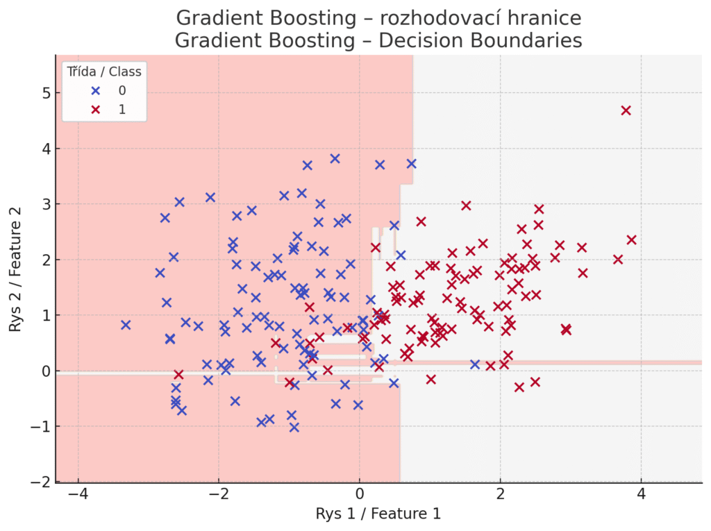
How the Gradient Boosting Classifier works – the coloured areas show the decision boundaries that arise as a result of the sequential training of trees, where each further model tries to improve on the previous one by learning from its errors. Unlike AdaBoost, the errors are not handled by weighting the samples but as gradients of the loss function, which the new models approximate. The model consists of several trees that are not independent but build on one another.
A comparison of the algorithms
Now that we have gone through the individual algorithms, let us look at how they compare in terms of accuracy, computational demands, interpretability and suitable data size.
| Algorithm | Quality/validation | The computational demand (training / inference) | The interpretability | Data size |
|---|---|---|---|---|
| Logistic Regression | Medium (a linear model) | Very low / very low | High (the weights are easy to explain) | Small and large (scales well) |
| Linear Regression | Medium (a linear model) | Very low / very low | High (the coefficients are easy to interpret) | Small and large (scales well) |
| Decision tree | Medium (a simpler model) | Low / low (fast decisions) | High (easily readable rules) | Small to medium (for large data an ensemble is better) |
| Random forest | High (an ensemble of trees) | Medium / medium (many trees) | Lower (many trees make it complicated) | Medium to large (scales with parallelisation) |
| KNN | Medium (depends on the data) | Negligible / grows with the size of the data | Low (hard to interpret, examples) | Small (large data = slow queries) |
| SVM | High (with a suitable kernel) | High / low-medium (demanding training, fast prediction with a small number of support vectors | Low (a black box for non-linear kernels) | Small to medium (large data = slow training) |
| Naive Bayes | Lower to medium (a simple model) | Very low / very low | Medium (the probability values are partly comprehensible) | Small and large (fast for any volume) |
| Artificial networks (ANN) | High to very high (depends on the architecture, the data and the tuning) | Very high / medium (demanding training, inference according to size) | Very low (not interpretable) | Rather large (they need a lot of data) |
| K-means | Silhouette, Davies-Bouldin index | Medium / low (iterative learning, fast Classification) | Low (the clusters have to be interpreted) | Medium to large (scales linearly) |
| SOM | Topological error, quantisation error | Medium / medium (O(n × epochs), fast Classification) | Low (the areas of the map are hard to interpret) | Medium (suitable for visualising medium-sized data) |
| PCA | Explained variance ratio | Medium (demanding with many features) / low | Low (the components are hard to explain) | Medium (very large data require approximate methods) |
| AdaBoost | High (improves weak models) | Medium / medium (a sequential ensemble) | Low (a combination of many weak models) | Small to medium (sensitive to noise in large data) |
| Gradient boosting | Very high (top performance) | High / medium (many iterations) | Low (a black-box ensemble) | Medium to large (optimised for large data) |
| └─ XGBoost | Very high | Medium-high / medium (an efficient C++ implementation) | Low (one has to use feature importance, for example) | Medium to large (the Kaggle standard) |
| └─ LightGBM | Very high | Low-medium / medium (highly optimised) | Low (similar to XGBoost) | Large (scales to massive data) |
(Note: “Quality/validation” for supervised methods denotes the general ability of a model to achieve a low error – the actual accuracy depends on the nature of the data. For unsupervised methods, specific metrics for evaluating the quality of the clustering or of the dimensionality reduction are given.)
Several trends can be seen from the table. Simple models such as logistic regression or a decision tree are fast and easy to understand, but they need not achieve the highest accuracy on complex problems. More complex models – ensembles of trees (random forest, boosting) and deep neural networks – usually offer higher accuracy, especially for large and complex datasets, but at the price of greater computational demands and a loss of interpretability. A deep neural network or XGBoost, for example, can uncover very complex relationships in a large volume of data and achieve top performance, but the resulting model is opaque to a human being and requires enough data and computing power for training. Conversely, models such as decision trees or logistic regression are suitable if we need an explainable model and have a rather small or medium dataset with a simpler structure.
Another important aspect is the computational demand of training vs. deployment. With most algorithms the most demanding phase is training (learning from the data), while prediction (inference) tends to be relatively fast. An SVM, for example, may train for a long time, but once the decision boundary has been found, the classification of Classification new points is a matter of computing scalar products with the support vectors – with a small number of support vectors this is fast, but with thousands of support vectors inference can be slower. Similarly, a neural network has to be trained iteratively over many epochs, but the resulting model can then predict in milliseconds to seconds (given sufficient hardware). The exception is KNN, where training is trivial (storing the data), but deployment requires comparison with the whole training set, so that as the data grow, prediction slows down. That is why KNN is suitable only for smaller volumes of data, or optimisations have to be used.
Interpretability vs. accuracy are often in opposition – simpler models (linear ones, trees) are more interpretable, while models with high capacity (ensembles, deep networks) provide higher accuracy at the price of a “black box”. This trade-off is well known, and in practice it is also addressed with explainable AI techniques (deriving feature importance, approximating a complex model with a simpler one and so on). From the point of view of the size of the data it can be said that for small datasets simpler models are more suitable – a complex model might learn them by heart (overfit) without any ability to generalise. Conversely, for very large datasets it is often essential to use models that can scale and exploit the potential of the data (LightGBM for tabular data, or deep networks for images and text). Some algorithms (an SVM with a non-linear kernel, or KNN) are not practical for millions of samples because of the computational load. In that case one chooses either a simpler version (a linear SVM, approximate KNN) or completely different methods.
So which algorithm should I actually use?
In machine learning there is no single universally best algorithm – the choice depends on the nature of the task, the available data and the requirements.
Perhaps the following guidance may help…
When I have little data and need easy interpretation
Start with logistic regression or a decision tree. These models give a fast response and their results can easily be explained in business terms. For a simple Classification (yes/no) with a few hundred records, logistic Regression will often be sufficient and will offer a clear view of the influence of the individual inputs. A decision tree, in turn, will help to reveal the key decision rules.
When every percentage point of accuracy on structured data matters
Try ensemble methods. Random forest is a good starting point – it often gives solid results without much tuning. If, however, you need maximum performance, reach for XGBoost or LightGBM. These gradient boosting models typically achieve the highest accuracy on tabular data. Bear in mind, though, the risk of overfitting – watch parameters such as the depth of the trees and the number of iterations, and use cross-validation to verify performance.
I have a lot of data and little time
If you have millions of rows and want to train a model quickly, LightGBM may be more suitable than a random forest or a classic SVM – LightGBM is designed to scale to large data and can handle even very bulky tasks. Also, linear models (linear Regression, logistic Regression or a linear SVM) can process large amounts of data quickly thanks to their simple functional form. Neural networks can also process large volumes, but training time and the need for tuning are factors that have to be taken into account.
For really complex data (images, text, sound) with many features
Here the field is usually ruled by deep neural networks. If you are solving a task of image or natural-language recognition, modern neural network architectures (CNN, RNN, Transformers) will as a rule offer the best results. Enough training data and computing resources are needed, however. For a quick start you can also use pre-trained models (transfer learning), so that everything does not have to be trained from scratch. In smaller projects an SVM or simpler models with hand-crafted features can be tried as a baseline, but in general deep learning leads in these domains.
When I do not know what I am looking for
If you have no training targets (labels), then use, for exploring the data and revealing structures, clustering or reduce the dimension. K-means is a good starting clustering algorithm if you have some idea how many groups to look for. For visualisation or data pre-processing, a good choice is PCA, or more advanced methods if the linearity of PCA is not enough. These techniques can help you understand the data better, find segments or prepare inputs for subsequent modelling.
How should we look at all this?
The choice of algorithm should be guided by experiments. The procedure recommended by experienced professionals is to try simpler interpretable models first, in order to gain a basic idea of the data and set a reference performance (a baseline). Then more complex algorithms can be tried and it can be verified whether they bring an improvement in performance.
At the same time, keep an eye on other circumstances and factors: if, for example, you need to deploy the model in real time on a device with limited performance, an overly complex model may be impractical. Conversely, for off-line analyses longer training may be acceptable.
Also important are maintenance and interpretation – in some applications (healthcare or finance, for instance) a simpler, explainable model may be preferred over a marginally more accurate but “opaque” one, because of trustworthiness and regulatory requirements.
In choosing the right algorithm we therefore weigh up the trade-offs between accuracy, complexity and comprehensibility. With practice and experience you will get a better sense of which type of model suits a given problem. This article has given you a basic overview and comparison, which may help beginning data enthusiasts to make an informed decision in their first machine-learning projects.
Modern trends in machine learning include AutoML for automatic hyperparameter tuning, explainable AI techniques (SHAP, LIME) for better interpretability of complex models, and stacking - an advanced ensemble method in which the outputs of different models serve as inputs for a meta-model. In practice, emphasis is also placed on the ethical aspects and fairness of models - metrics such as Equal Opportunity or Demographic Parity, with tools such as Fairlearn in Python - and on their transparency, especially in sensitive areas such as healthcare and finance.An overview of the basic machine-learning algorithms in a table
| Algorithm | Advantages | Disadvantages | Additional notes |
|---|---|---|---|
| Logistic Regression | Less prone to overfitting, fast training. Excellent interpretation (odds ratio, p-values). | With high-dimensional data it can overfit and it suffers from multicollinearity. It assumes a linear relationship between the log-odds and the inputs. | Suitable as a “baseline” for binary/multi-class classification, works well with regularisation (L1/L2). |
| Linear Regression | Extremely fast, the coefficients are easy to interpret. Regularisation (Ridge/Lasso) reduces overfitting. | Strong assumptions (linearity, homoscedasticity, normality of the residuals). Sensitive to outliers and noise. | Suitable for estimating a continuous quantity with a linear dependence; for non-linearity the features have to be extended or polynomials added. |
| Decision tree | Solves non-linear problems, handles both numerical and categorical features. Easy visualisation and explanation. | High risk of overfitting; a small change in the data leads to a different tree. Bias towards attributes with many levels. | Overfitting is dampened by pruning, bagging or a Random Forest. |
| Random forest | High accuracy thanks to the ensemble, resistant to noise. Estimates feature importance, overfits less than a single tree. | Limited interpretability (hundreds of trees), higher computational demands than a single tree. | Popular for tabular data, with built-in feature importance for feature selection. |
| K-NN | A “lazy learner” – no learning phase, simple. Usable for both classification and regression. | Scales badly to large datasets, memory-intensive. Sensitive to feature scale, to noise and to the choice of K. | In practice it is combined with indexed or approximate search (KD-tree, FAISS). |
| SVM (Support Vector Machine) | Excellent for high-dimensional data and small samples. Kernel tricks give non-linear decision boundaries. | Training is O(n²-n³), unsuitable for millions of samples. Sensitive to the choice of kernel, C and γ; hard to interpret. | LinearSVM (+SGD) solves the scaling; careful standardisation of features is necessary. |
| Naive Bayes | Very short training, works even with a small amount of data. Popular for text classification (high dimension). | A strong (often violated) assumption of the conditional independence of features. The zero-frequency problem (solved by Laplace smoothing). | Surprisingly competitive if the features are more or less independent. |
| ANN (artificial neural networks) | Can model complex non-linear relationships. Good generalisation, the possibility of parallelisation on GPU/TPU. | Long training and numerous hyperparameters. A “black box” – low interpretability, requires a large amount of data. | Modern frameworks (PyTorch, TensorFlow) make development easier; explainability is addressed by SHAP, LIME and similar tools. |
| K-means (clustering) | Simple, fast and scalable. Guaranteed convergence to a local minimum. | Sensitive to outliers and to the initial centroids. The choice of K is often not obvious (Elbow, Silhouette). | It assumes spherical clusters; for other shapes DBSCAN or a GMM can be chosen. |
| SOM (Self-Organizing Maps) | Preserves topology, excellent visualisation of complex data, relatively fast training O(n × epochs). | Sensitivity to the choice of grid size and initial weights, difficult interpretation of the areas of the map. | Exclusively an exploratory tool for visualising and segmenting high-dimensional data. |
| PCA (principal component analysis) | Reduces correlated features, giving a lower dimension and less overfitting. Speeds up subsequent models. | The components are hard to interpret. Loss of information is unavoidable; standardisation is required. | Often a step before classification/regression or visualisation (2D/3D). |
| AdaBoost | The ensemble approach increases accuracy and dampens overfitting. Simple implementation (weak learners + weights). | Highly sensitive to noise and outliers. Its sequential character makes it slower than bagging. | The most common weak learner is a stump (a one-level tree). |
| Gradient boosting (XGBoost, LightGBM) | Top accuracy on tabular data, an efficient implementation with parallelisation and regularisation. | Higher computational demands, many hyperparameters to tune, a black-box model. | Dominates Kaggle competitions, often the go-to choice for structured data in industry. |
Article licence: This article is licensed under Creative Commons. You may freely share and adapt it provided you credit the author and link to this text.


